In today’s power systems, many short- and long-term decisions depend on the forecasts of solar and wind generation. Consequently, millions of dollars have been poured into the development of cutting-edge forecasting tools, designed to predict the output of these renewable energy sources, which hinge on weather conditions.
Although numerous sophisticated forecasting methods have emerged to enhance the accuracy of these predictions, they all share one fundamental constraint: the “inherent predictability” of the data used. In this context, predictability refers to the ability to determine, ahead of time, the availability of a generation resource [1]. When the predictability of a renewable resource is low, forecasting errors become more likely, whereas high predictability makes forecasting easier, regardless of the model employed.
Interestingly, our recent analysis of PV generation and solar irradiance data from Australia revealed that predictability can vary dramatically across different locations and times. This variability in predictability has far-reaching implications, as it can lead to additional charges for renewable plants and pose technical challenges for grid operations.
Recognising this, it becomes essential to incorporate predictability into relevant decision-making processes. By doing so, we can optimise the integration of renewables into the grid, reduce costs, and maintain a reliable power system.
How can we measure predictability?
While lower forecast errors could imply higher predictability in a given time series, they cannot be used as a surrogate parameter for predictability for many reasons. In our recently published research paper, we presented a new methodology for quantifying renewable data predictability, using weighted permutation entropy (WPE).
We define the predictability index as 1-WPE, where a lower WPE indicates higher predictability, and vice versa. In the following, we provide several examples of how using this metric can improve power system decisions.
Application 1: Private investment decisions
When finding the optimal location for constructing solar and wind farms, various factors — such as solar or wind energy atlases, geographic information system (GIS) data, transmission networks, and road access — are taken into account. The chosen location has significant implications on investment costs, energy yields, and even the facility’s participation in day-ahead and/or spot electricity markets.
Like conventional power plants, solar and wind farms face financial penalties for deviating from their market commitments. Such deviations are more likely for renewable plants, as their “fuel” depends on weather conditions. Consequently, errors in renewable generation forecasts can result in supply-demand imbalances within the power grid and financial penalties for renewable plants. For instance, in the Australian National Electricity Market (NEM), the operator uses regulation Frequency Control Ancillary Services (FCAS) to ensure the balance between supply and demand. The Australian Energy Market Operator (AEMO) then recovers the regulation FCAS costs from market participants by determining how much each has contributed to the need for this service, called the Causer Pays procedure. Figure 1 shows the share of regulation FCAS charges per terawatt-hour of produced energy for the NEM power plants based on fuel types in each quarter of 2020. While the total production (and hence revenue) of solar PV and wind farms was much less than coal- and gas-fired plants, the share of regulation FCAS charges for renewable plants was considerably higher than those for conventional power plants.
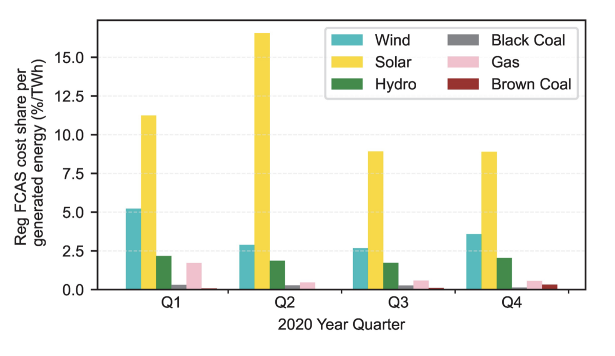
Image: Sahand Karimi / University of Adelaide
The main reason for higher regulation FCAS charges among solar farms is the significant prediction errors in their generation forecasts, which lead to higher Causer Pay factors (CPFs), based on which a specific percentage of the regulation FCAS costs are assigned to each power plant. Figure 2 depicts the relationship over time between the CPFs of six solar farms in New South Wales (NSW) and the predictability of PV generation in 2019. The predictability is determined based on two different datasets: 1) the historical generation of 100+ rooftop PV systems in NSW, obtained from Solar Analytics, and 2) five minute historical data of global tilted irradiance (GTI) at the six solar farm locations, downloaded from SolCast.
The figures demonstrate a strong negative correlation between the average CPF, and the predictability for the actual solar generation and the GTI of solar farms. This means when the generation predictability of a solar farm was higher, its CPF was lower. As the CPF is directly related to regulation FCAS charges, it is clear that higher predictability of generation would result in lower regulation FCAS costs allocated to the renewable plant.
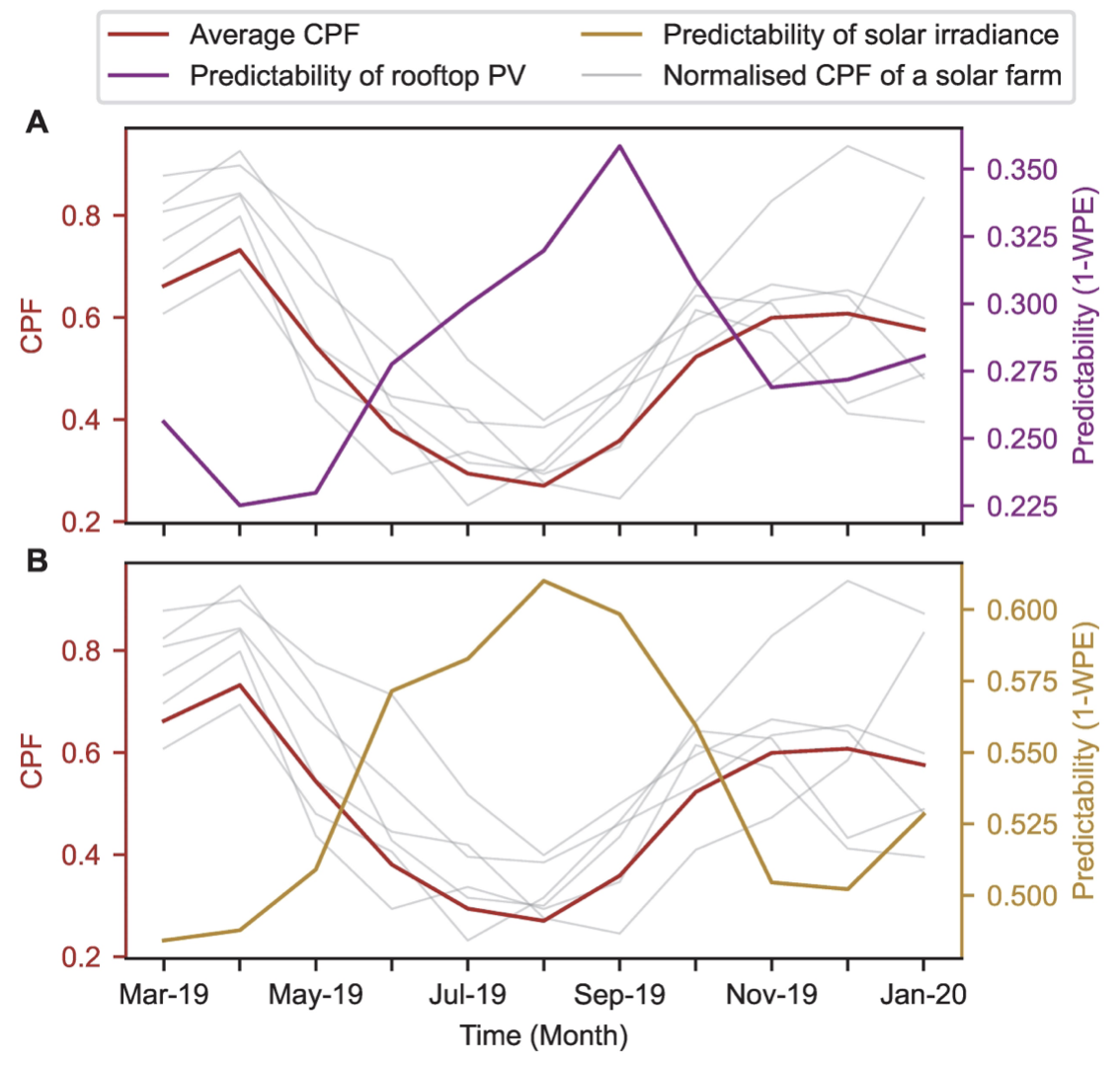
Image: Sahand Karimi / University of Adelaide
To quantify the monetary value of predictability, we estimated how much the CPF of a solar farm would decrease when there is a specific amount of increase in its predictability. The scatter plots in Figure 3.A illustrate the vivid relationship between the average predictability and the CPF of solar farms over two-month rolling windows. We further validated the results by analysing the relationship between the annual predictability of solar farms’ irradiance and their average CPF for a year in Figure 3.B.
In all scatter plots, the correlation was statistically significant, indicating a strong negative correlation between predictability and CPF. Additionally, the slope of the regressed lines is similar in all three cases, suggesting a robust relationship exists between the CPF and the predictability for the studied period. Using the most conservative estimate for the relationship between the CPF and the predictability, we could estimate a 0.1 increase in the predictability would reduce CPF by 0.272. Given that the average annual cost of the regulation market was about $85.6 million (USD 56.6 million) in the last five years, a 0.272 reduction in the CPF leads to roughly $233,000 lower cost of regulation FCAS each year.
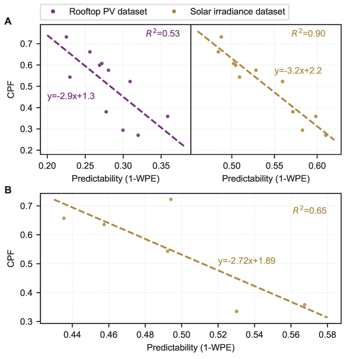
Image: Sahand Karimi / University of Adelaide
Figure 4 illustrates the changes in the predictability of solar PV generation in various locations in Australia. We can observe that the PV generation predictability varies significantly across different regions and even within each state, indicating that it is highly location-dependent. Based on the previous analysis, we can estimate that a 100 MW solar farm could lose roughly $900,000 of its revenue each year because of these differences in PV generation predictability (this would be 9% of its potential $10 million revenue).
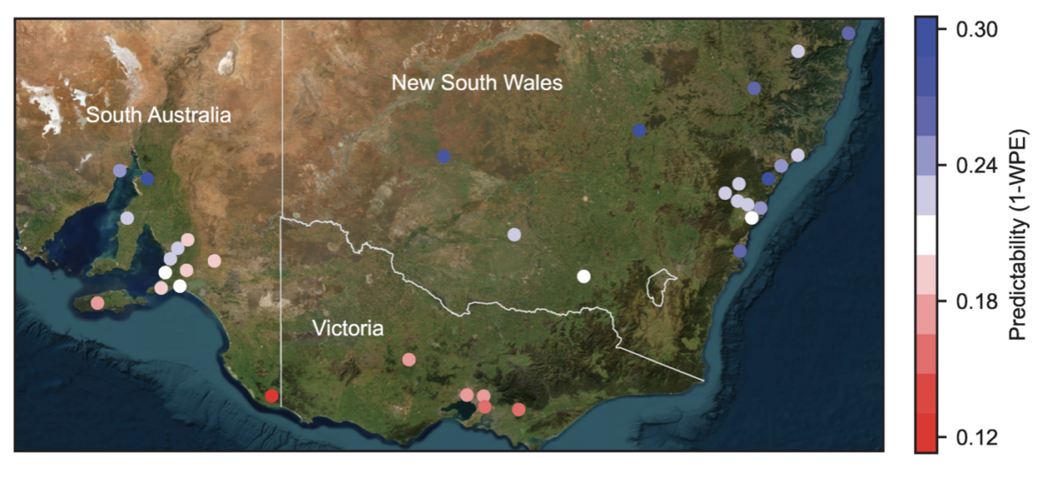
Image: Sahand Karimi / University of Adelaide
Case study of nine solar farm locations
To better understand the impact of considering PV generation predictability on the decision to build a solar farm, we conducted a case study on nine potential locations in NSW, shown in Figure 5. Our goal was to determine the best location for a hypothetical 51.8 MW solar farm in two different scenarios (51.8 is the average of six solar farms’ capacity from the previous analysis).
In the first scenario, the projected revenue of the solar farm was calculated based on the total solar energy yield, which is typically considered the main factor for estimating future revenue. In the second scenario, we considered both the revenue and the Causer Pays costs in calculating the projected net revenue of the farm.
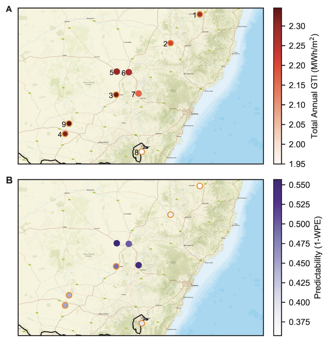
Image: Sahand Karimi / University of Adelaide
To compare the expected net revenue of the solar farm in different locations for the two scenarios, we used the GTI sun-tracking data of locations shown in Figure 5 from August 2021 to August 2022. We set location 1, where the White Rock solar farm is installed, as our baseline in the comparison.
Based on the historical data, the White Rock solar farm had an annual revenue of about $10,000 per MW installed capacity in 2020. Accordingly, we calculated the revenue of a 51.8 MW solar farm in other locations, assuming a 1% higher annual GTI would lead to 1% more revenue. Also, we used the quantitative relationship between the predictability and CPF, mentioned in the previous analysis, to estimate the monetary value of better predictability.
Finally, the net revenue of the solar farm in different locations is compared in Figure 6. As seen in the figure, location nine would be the best option for building a 51.8 MW solar farm without considering the predictability.
However, if the cost associated with the predictability of PV generation were taken into account, location five would be the best option by a significant margin over location nine. Once predictability is considered in the solar farm investment decision, the ranking of the choices changes significantly in relation to the highest net revenue. These findings indicate the generation predictability of renewable plants has a material impact on their profit.
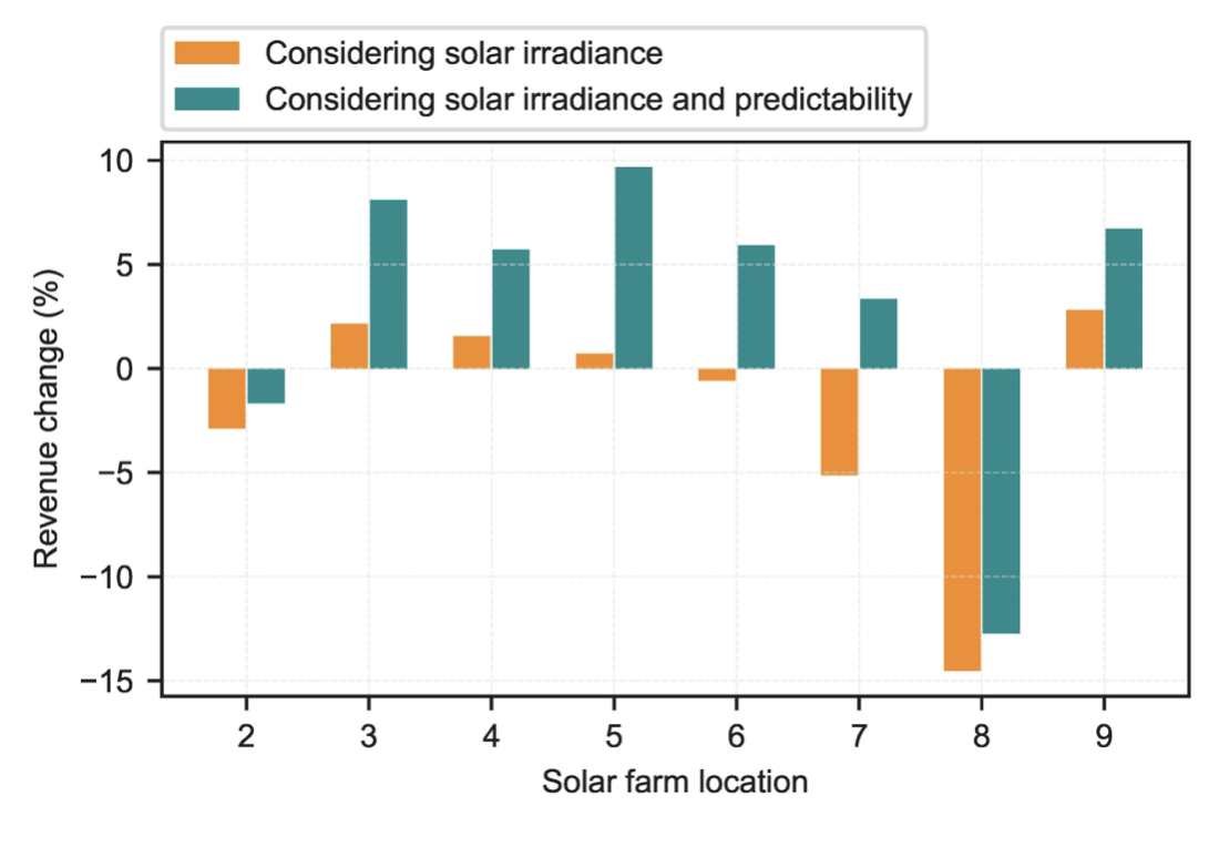
Image: Sahand Karimi / University of Adelaide
To find the best locations for future solar and wind farm projects, we need to take into account the cost implications of their resource predictability as a decisive factor, in addition to the other technical and financial factors currently being used. This can be done by measuring the predictability of the potential renewable generation at a location, using the existing (or simulated) generation data or relevant surrogate variables, such as GTI for solar farms.
Application 2: Policy design
The unpredictability of renewable generation, caused by inherently uncertain weather forecasts, has increased the costs of reserve electricity markets. For instance, the UK power grid experiences a 5 to 10 British Pounds per MWh increase in the reserve market costs for 1 MW additional wind or solar production due to their prediction errors. As the number of renewable plants increases in the electricity grid, the additional cost of operational reserve requirements per MWh of renewable energy will rise even more. Given that consumers (or taxpayers) pay for these costs on their electricity bills (or government subsidies), governments are responsible for minimising these costs through well-planned investments and shrewd policy design.
In November 2021, South Australia (SA) became the first gigawatt-scale power grid in the world to reach zero net demand when the combined output of rooftop solar and other small-scale generators exceeded the total customers’ load demand. This has been achieved mainly by the federal government’s subsidies on rooftop PV panels as well as state government policies. Despite all the benefits, the high level of distributed PV generation has led to higher variability of power system net demand, which can cause high spot energy prices, voltage swings, or even loss of supply if not adequately managed. One well-known solution is to integrate costly battery storage systems in the grid. Yet, a cheaper but effective way to mitigate some of these issues is to invest in renewable energy sources with higher generation predictability.
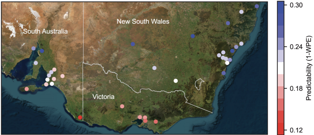
In this regard, recognising the differences in the predictability of renewable generation in different areas could change the public sector policies for the better long-term. For instance, as shown in Figure 7, northern SA with the highest predictability has an average density of rooftop PV systems equal to 41.5%, comparable with the south (40%) with significantly lower predictability. A better policy could have been offering different incentives in different regions based on their predictability, e.g., rooftop PV only in the northern part of the state and PV plus battery in the south.
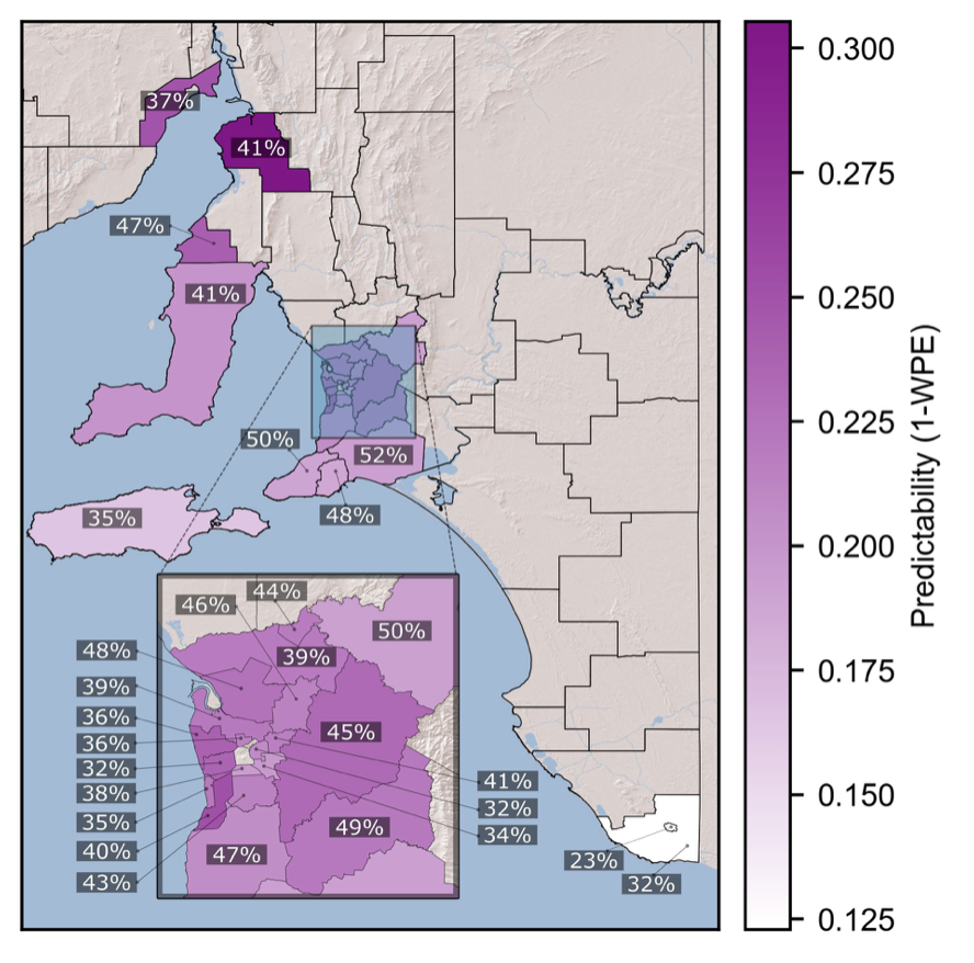
Image: Sahand Karimi / University of Adelaide
On a larger scale, considering the predictability of renewable resources as a factor in the decision-making processes can enhance strategies for incorporating increased levels of renewable energy generation. For instance, the lower predictability of PV generation in Victoria suggests increasing rooftop solar in that region will increase net demand (operational demand) uncertainty compared to other states, which in turn requires a higher amount of operational reserve requirements in the power grid; hence, higher cost of energy for consumers. This can shape the policies and regulations to push for alternative renewable generation (e.g., small-scale wind turbines) instead of rooftop PV or subsidies on home battery systems in that region.
Application 3: Power system operation and planning
Looking into the predictability variations over time reveals interesting seasonality patterns in solar generation predictability that can be useful in power system planning and operation.
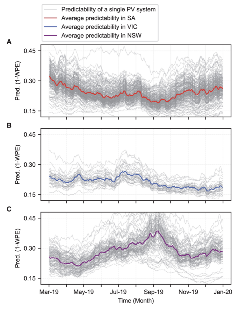
Image: Sahand Karimi / University of Adelaide
Figure 8 presents the predictability profiles of the rooftop PV generation in three Australian states: NSW, Victoria and SA. In these figures, each line represents the predictability profile of an Australian household rooftop system over the year 2019, calculated based on two-month rolling windows.
It can be seen that the evolution of predictability over time varies remarkably from one state to another. This finding has potential applications in power systems planning, e.g., to jointly plan future flexibility resources (such as batteries or pumped hydro storage) and interconnections between states to share flexibility capacity in different seasons. For example, the PV generation predictability is the lowest in NSW during the summer while the highest in SA during the same period. In the event of proper interconnection between the two states (e.g., through the incoming interconnector), the flexible assets, such as batteries, in SA can assist in managing the higher renewable generation unpredictability in the NSW grid.
The average predictability of solar generation in each state can also inform power system operators and market participants in determining the time frame for the annual maintenance of their assets, ensuring the availability of enough reserve requirements when renewable resources have lower predictability. Lastly, acknowledging that the maximum capability of forecast methods varies in different states over time can advise power system operators regarding the forecasting accuracy of renewable sources in different areas; thus, better estimations for required frequency regulation requirements in the system.
Concluding remarks
In most electricity markets, renewable plants are currently subject to different rules than conventional ones. For example, in the NEM, conventional generators (categorised as “scheduled”) are non-compliant with the rules if their generation deviates from the instructed dispatch targets considerably; renewable plants (categorised as “semi-scheduled”) are not. As most coal power plants are expected to retire in the next few years, the existing market rules are going through massive changes to ensure reliable grid operation. Such changes could imply if renewable plants’ generation were not predictable, they would need to maintain sufficient headroom to accommodate unpredictable generation changes and meet their forecasts. This would of course result in spilling a high portion of their clean energy and earning less revenue. Selecting locations with high renewable resource predictability for future renewable projects will minimise these risks.
As electricity generation and consumption undergo significant transformations, both are becoming increasingly unpredictable. As a result, accurately estimating and considering the predictability of renewable resources has become more crucial than ever. Although forecasting models play an essential role, they will never be perfect. Therefore, it is vital to address the other half of the problem: the inherently limited predictability of intermittent generation sources. By measuring this property of renewable resources, policymakers, investors, power system planners and operators, and third-party service providers in the electricity industry can gain valuable insights for improved decision-making.
–
About the author
Sahand Karimi is a PhD candidate at the University of Adelaide and CSIRO Energy, where he focuses on developing novel battery solutions for solar and wind farms. Since 2017, he has been working on research, analysis, and modelling of various problems in power systems and electricity markets. Alongside his academic research, Sahand currently works as a Power System Engineer at the Australian Energy Market Operator (AEMO).
–
[1] Managing large-scale penetration of intermittent renewables. MIT Energy Initiative (2012). URL: https://energy.mit.edu/wpcontent/uploads/2012/03/MITEI-RP-2011-001.pdfThe views and opinions expressed in this article are the author’s own, and do not necessarily reflect those held by pv magazine.
This content is protected by copyright and may not be reused. If you want to cooperate with us and would like to reuse some of our content, please contact: editors@pv-magazine.com.


By submitting this form you agree to pv magazine using your data for the purposes of publishing your comment.
Your personal data will only be disclosed or otherwise transmitted to third parties for the purposes of spam filtering or if this is necessary for technical maintenance of the website. Any other transfer to third parties will not take place unless this is justified on the basis of applicable data protection regulations or if pv magazine is legally obliged to do so.
You may revoke this consent at any time with effect for the future, in which case your personal data will be deleted immediately. Otherwise, your data will be deleted if pv magazine has processed your request or the purpose of data storage is fulfilled.
Further information on data privacy can be found in our Data Protection Policy.